
꺼내먹는지식 준
MLP (neural)CF, AutoRec 코드 구현 간단 정리 본문
MLP NCF
neural collaborative filtering 에 맞는 형태로 데이터를 변환
ratings_df = pd.read_csv(data_path + 'u.data', sep='\t', encoding='latin-1', header=None)
ratings_df.columns = ['user_id', 'movie_id', 'rating', 'timestamp']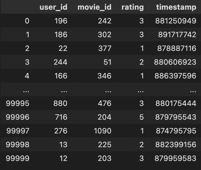
user_ids = ratings_df['user_id'].unique()
movie_ids = ratings_df['movie_id'].unique()
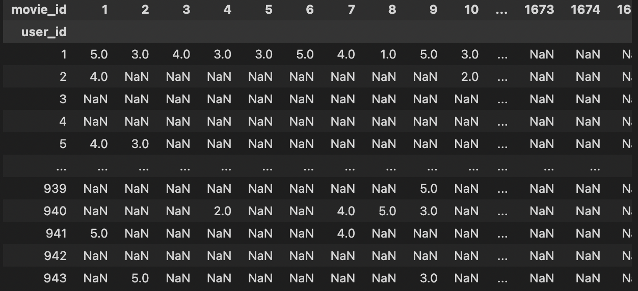
ratings_matrix = ratings_df.pivot(index='user_id', columns='movie_id', values='rating')
#pivot 함수, index(각 행의 label), columns(각 열의 label), values굉장히 유용한 df.pivot 함수
한번에 column, index, 그리고 value 까지 원하는 값으로 정리 가능
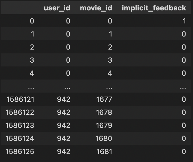
#implicit_feedback
implicit_df = dict()
implicit_df['user_id'] = list()
implicit_df['movie_id'] = list()
implicit_df['implicit_feedback'] = list()


user_dict = dict()
movie_dict = dict()


for u, user_id in tqdm(enumerate(user_ids)):
    user_dict[u] = user_id
    #연속적인 순서를 key, value 는 user_id
    for i, movie_id in enumerate(movie_ids):
        if i not in movie_dict:
            movie_dict[i] = movie_id
        #user_dict, movie_dict 는 lookup table 느낌
        implicit_df['user_id'].append(u)
        implicit_df['movie_id'].append(i)
        #implicit_df 의 user_id 와 movie_id 는 lookup table 의 key 값
        if pd.isna(ratings_matrix.loc[user_id, movie_id]):
            #iloc 은 index, loc 은 이름
            #여기서는 user_id, movie_id 이름으로 뽑아야 하니까 loc
            implicit_df['implicit_feedback'].append(0)
            #Nan 인 경우에는 0
        else:
            implicit_df['implicit_feedback'].append(1)
            #본적 있는거면 점수에 상관없이 1
implicit_df
user_id, movie_id 가 지저분해서 look up table 로 정리하기 위하여 enumerate 사용
pd.isna 함수로 NaN을 0으로 치환 0, 1~5의 rating은 1
train_X, test_X, train_y, test_y = train_test_split(
    implicit_df.loc[:, implicit_df.columns != 'implicit_feedback'], implicit_df['implicit_feedback'], test_size=0.2, random_state=seed,
    stratify=implicit_df['implicit_feedback']
)implicit_df.columns
Index(['user_id', 'movie_id', 'implicit_feedback'], dtype='object')implicit_df.columns != 'implicit_feedback'
array([ True, True, False])implicit_df.loc 에 어떻게 적용되는 건지에 대한 확인이 필요
※pandas tip
- loc 은 index, column value 의 명칭 으로 indexing
- iloc 은 index, column 의 index 로 indexing
implicit_df.loc[:, ('user_id', 'movie_id')]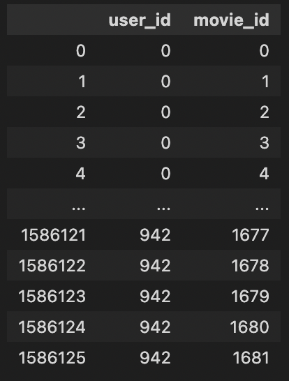
implicit_df.loc[:,[True, True, False]]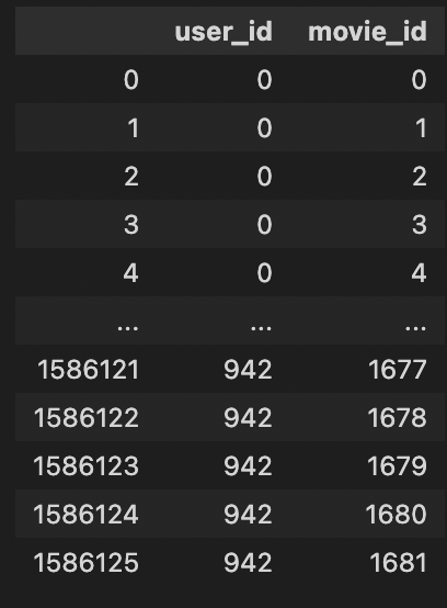
정리하자면, loc은 boolean 으로 indexing 이 가능하다.
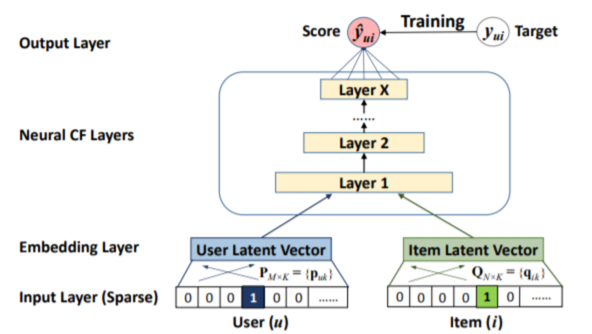
MLP에 넘겨주기 위하여 user, item embedding 을 concatenate 한다.
MLP layer 를 선언하는 부분이 흥미롭다.
self.mlp_layers = MLPLayers([2 * self.emb_dim] + self.layers, self.dropout) #layer: [256, 64]다음과 같이 선언하면 추후, layer 의 개수에 변화를 주고 싶을 때 얼마든지 자유롭게 변화를 줄 수 있다.
여기서는 [256, 64] 로 hidden의 크기가 줄어든다.
(1024, 256) (256, 64) (64, 1) 총 2개의 hidden 과 1개의 최종 layer
parameter 초기화
def _init_weights(self, module):
    if isinstance(module, nn.Embedding):
        normal_(module.weight.data, mean=0.0, std=0.01)
    elif isinstance(module, nn.Linear):
        normal_(module.weight.data, 0, 0.01)
        if module.bias is not None:
module.bias.data.fill_(0.0)self.apply(self._init_weights)apply 는 sequential 로 연결된 모든 layer 를 한방에 recursive하게 초기화해준다.
해당 방법이 익숙하지 않아서 왜인가 했더니
파이토치에서는 기본적인 모듈 클래스(Linear, ConvNd 등) 를 초기화 할 때, 자동으로 파라미터를 적절히 초기화 해 주고 있고
또한 각 모듈 내의 reset_parameters() 메소드만 호출해 주면 어렵지 않게 모듈 파라미터를 초기화 할 수 있기 때문이다.
※ 참고
import torch

layer = torch.nn.Conv2d(1, 1, 2)

# Normal distribution
torch.nn.init.normal_(layer.weight)

# Xavier initialization
torch.nn.init.xavier_uniform_(layer.weight)

# Kaiming initialization
torch.nn.init.kaiming_uniform_(layer.weight)
아래와 같이 xavier 을 많이 사용한다.
def weight_init_xavier_uniform(submodule):
    if isinstance(submodule, torch.nn.Conv2d):
        torch.nn.init.xavier_uniform_(submodule.weight)
        submodule.bias.data.fill_(0.01)
    elif isinstance(submodule, torch.nn.BatchNorm2d):
        submodule.weight.data.fill_(1.0)
        submodule.bias.data.zero_()
정리해보면,
input_feature = torch.cat((user_e, item_e), -1)
mlp_output = self.mlp_layers(input_feature)
output = self.predict_layer(mlp_output)
output = self.sigmoid(output)
다음과 같이 user embedding, item embedding 을 concat 하고 mlp 통과시킨 후 sigmoid 로 얻은 output을 RMSE loss 를 사용한다. mlp 는 각 hidden layer 전에 dropout 을 넣기도 한다.
 for batch, (X, y) in enumerate(dataloader):
        X, y = X.to(device), y.to(device)
        # Compute prediction and loss
        pred = model(X)
        loss = loss_fn(pred, y)
        train_loss += loss.item()

        # Backpropagation
        optimizer.zero_grad()
        loss.backward()
        optimizer.step()
모델을 학습시킨다.
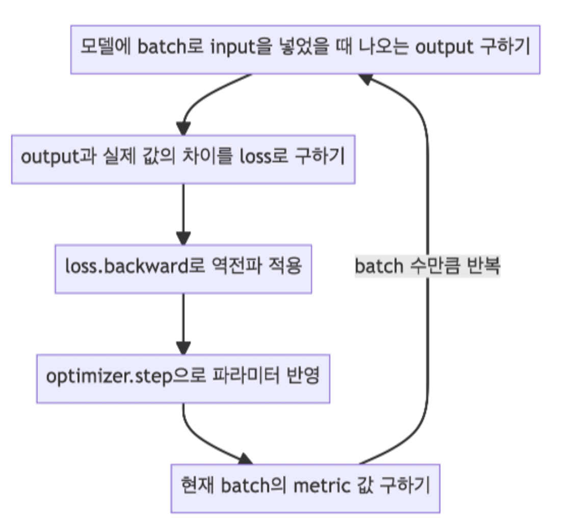
optimizer.zero_grad() 와 loss.backward(), optimizer.step() 을 한번만 더 정리해본다.
※ zero_grad()
: 보통 딥러닝에서는 미니배치+루프 조합을 사용해서 parameter들을 업데이트한다.
이 때 한 루프에서 업데이트를 위해 loss.backward()를 호출하면 각 파라미터들의 .grad 값에 변화도가 저장이 된다.
이후 다음 루프에서 zero_grad()를 하지않고 역전파를 시키면 이전 루프에서 .grad에 저장된 값이 다음 루프의 업데이트에도 간섭을 해서 원하는 방향으로 학습이 안된다.
따라서 루프가 한번 돌고나서 역전파를 하기전에 반드시 zero_grad()로 .grad 값들을 0으로 초기화시킨 후 학습을 진행해야 한다.
그럼 이 기능은 왜 존재할까?
gradients을 더해주는 방식은 RNN을 학습시킬때 매우 편리한 방식이라고 한다.
loss.backward() , optimizer.step()
# parameters에 대한 gradients 구하기
# 직접 미분 수식을 입력해주는 것과 같은 효과 (Autograd)
loss.backward() # loss를 w(가중치)로 편미분한다.

# update parameters
# 원래의 weight/bias에서 lr * gradients를 뺀 값으로 업데이트
optimizer.step() # w = w - lr * grad
AutoRec
대부분 상단에서 정리되어 추가적으로 언급할 내용이 적다.
하지만 데이터 전처리에서 차이를 보이는데, MLP 의 경우 rating 을 1, 0 binary 처리하여 학습하였다.
binary 로 처리한건 그냥 구현상 편리 같고, 0, 1, 2, 3, 4, 5 로 multi class classification 으로 풀어도 되지 않았나 싶다. (multi-class 는 cross-entropy)
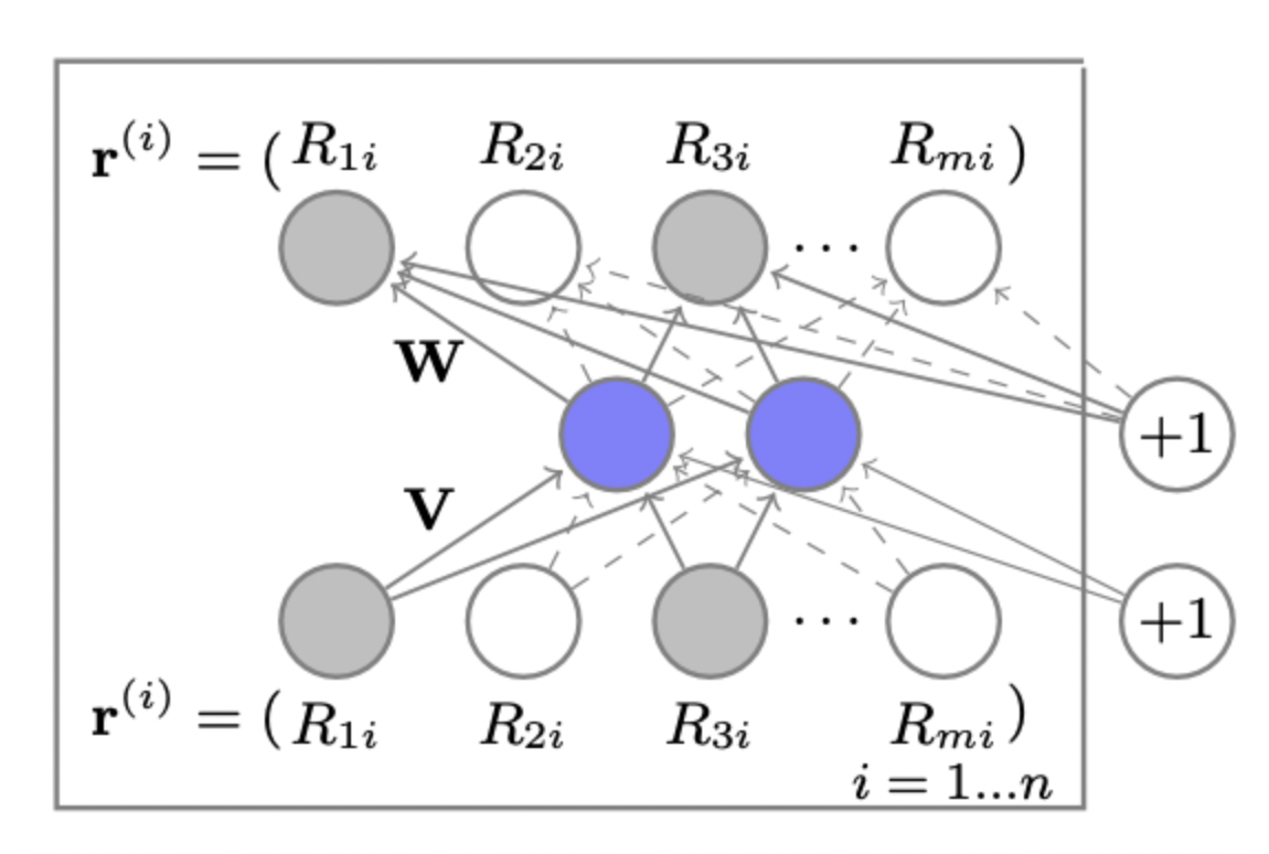
AutoRec 은 말그대로 input을 embedding 하고 다시 복원하는 기법이다.
user 가 평가하지 않은 영화의 NaN 은 0으로 치환
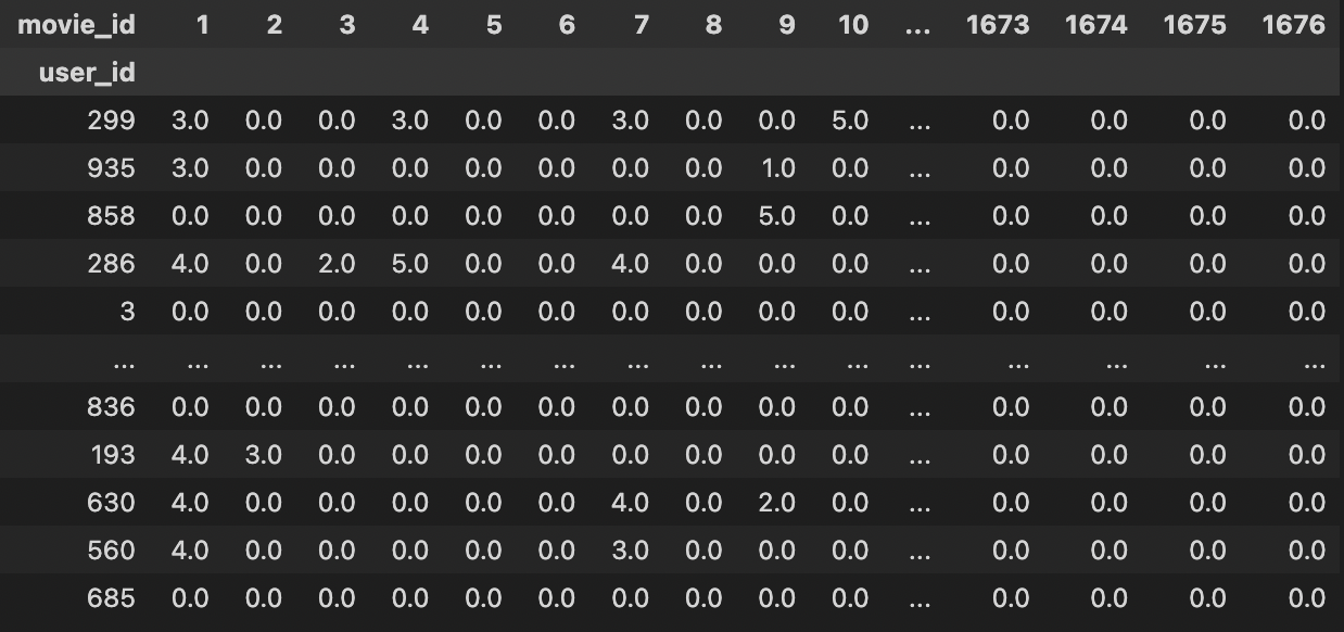
다음과 같은 데이터를
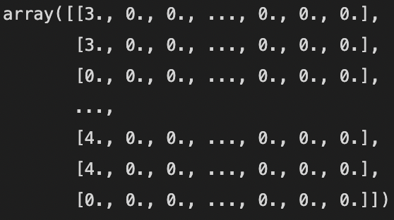
이와 같은 형태로, 즉 rating 점수로 하여 train set, test set을 만든다.
self.encoder =  nn.Linear(self.input_dim, self.emb_dim) # FILL HERE : USE nn.Linear() #
self.hidden_activation_function = activation_layer(hidden_activation)
self.decoder =  nn.Linear(self.emb_dim, self.input_dim)  # FILL HERE : USE nn.Linear() #
self.out_activation_function = activation_layer(out_activation)


def forward(self, input_feature):
    h = self.encoder(input_feature) # FILL HERE : USE self.encoder() # 128(batch), 1682  X 1682 512
    h = self.hidden_activation_function(h)

    output = self.decoder(h) # FILL HERE : USE self.decoder() #
    output = self.out_activation_function(output)

    return output
들어온 input (batch_size, 1682) 를 512 크기로 embedding 한다.
activation 은 relu 로 선택
그 후 decoder 는 복원 한다.
y_for_compute = y.clone().to('cpu')
index = np.where(y != 0) # FILL HERE : USE np.where & y_for_compute. WARNING: y를 사용 시, y의 device가 gpu일 경우 오류 발생 #
loss = self.loss_fn(pred[index], y[index])
복원한 값으로 loss 를 구한다.
np.where 에서 조건을 만족할 때의 결과를 따로 정해주지 않으면 각 차원의 index 를 return 해주고 이를 편리하게 index 로 바로 사용할 수 있다.
$$\underset{\theta}{min} \sum^{n}_{i=1} ||r^{(i)} - h(r^{(i)}; \theta) ||^2_{O}$$
여기까지 했을 때 이해가 잘 안가는 부분이 있다. 비단 Rating 값들을 embedding 하고 복원하는 과정이 어떤 의미가 있을까?
정리해보자면, 각 유저가 평가한 영화에 대한 서로 다른 rating 이 input으로 들어가고, 각 유저의 rating 을 복원하는 과정에서 반복 학습이 되면 우선적으로 representation vector 가 잘 만들어질 것으로 보인다.
그리고 약간 오염된 user data 가 복원이 잘 되도록 할 때도 사용할 수 있을 것 같다. (노이즈 낀 이미지 처럼)
'AI > 추천시스템' 카테고리의 다른 글
| 딥러닝 추천 모델 - 2 (Autoencoder) (0) | 2022.07.25 |
|---|---|
| 딥러닝 추천 모델 - 1 (MLP) (0) | 2022.07.24 |
| ANN (Approximate Nearest Neighbor) (0) | 2022.07.19 |
| Item2Vec (0) | 2022.07.19 |
| Collaborative Filtering - 2 (Model based CF, Matrix Factorization, Bayesian Personalized Ranking) (0) | 2022.07.15 |


